Standard deviation and variance are statistical measures of dispersion of data, i.e., they represent how much variation there is from the average, or to what extent the values typically “deviate” from the mean (average). A variance or standard deviation of zero indicates that all the values are identical.
Variance is the mean of the squares of the deviations (i.e., difference in values from the mean), and the standard deviation is the square root of that variance. Standard deviation is used to identify outliers in the data.
Important Concepts
- Mean: the average of all values in a data set (add all values and divide their sum by the number of values).
- Deviation: the distance of each value from the mean. If the mean is 3, a value of 5 has a deviation of 2 (subtract the mean from the value). Deviation can be positive or negative.
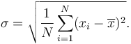
Symbols
The formula for standard deviation and variance is often expressed using:
- x̅ = the mean, or average, of all data points in the problem
- X = an individual data point
- N = the number of points in the data set
- ∑ = the sum of [the squares of the deviations]
Formulae
The variance of a set of n equally likely values can be written as:

The standard deviation is the square root of the variance:
Formulae with Greek letters have a way of looking daunting, but this less complicated than it seems. To put it in simple steps:
- find the average of all data points
- find out how far each point is away from the average (this is the deviation)
- square each deviation (i.e. the difference of each value from the mean)
- divide the sum of the squares by the number of points.
That gives the variance. Take the square root of the variance to find the standard deviation.
Example
Let’s say a data set includes the height of six dandelions: 3 inches, 4 inches, 5 inches, 4 inches, 11 inches, and 6 inches.
First, find the mean of the data points: (3 + 4 + 5 + 4 + 11 + 7) / 6 = 5.5
So the mean height is 5.5 inches. Now we need the deviations, so we find the difference of each plant from the mean: -2.5, -1.5, -.5, -1.5, 5.5, 1.5
Now square each deviation and find their sum: 6.25 + 2.25 + .25 + 2.25 + 30.25 + 2.25 = 43.5
Now divide the sum of the squares by the number of data points, in this case plants: 43.5 / 6 = 7.25
So the variance of this data set is 7.25, which is a fairly arbitrary number. To convert it into a real-world measurement, take the square root of 7.25 to find the standard deviation in inches.
The standard deviation is about 2.69 inches. That means that for the sample, any dandelion within 2.69 inches of the mean (5.5 inches) is ‘normal’.
Why Square the Deviations?
Deviations are squared to prevent negative values (deviations below the mean) from canceling out the positive values. This works because a negative number squared becomes a positive value. If you had a simple data set with deviations from the mean of +5, +2, -1, and -6, the sum of the deviations will come out as zero if the values aren’t squared (i.e. 5 + 2 – 1 – 6 = 0).
Real World Applications
Variance is expressed as a mathematical dispersion. Since it’s an arbitrary number relative to the original measurements of the data set, it is difficult to visualize and apply in a real-world sense. Finding the variance is usually just the final step before finding the standard deviation. Variance values are sometimes used in finance and statistical formulas.
Standard deviation, which is expressed in the original units of the data set, is much more intuitive and closer to the values of the original data set. It is most often used to analyze demographics or population samples to gain a sense of what is normal in the population.
Finding outliers

A normal distribution (Bell curve) with bands corresponding to 1σ
In a normal distribution, about 68% of the population (or values) falls within 1 standard deviation (1σ) of the mean and about 94% fall within 2σ. Values that differ from the mean by 1.7σ or more are usually considered outliers.
In practice, quality systems like Six Sigma attempt to reduce the rate of errors so that errors become an outlier. The term “six sigma process” comes from the notion that if one has six standard deviations between the process mean and the nearest specification limit, practically no items will fail to meet specifications.[1]
Sample Standard Deviation
In real world applications, data sets used usually represent population samples, rather than entire populations. A slightly modified formula is used if population-wide conclusions are to be drawn from a partial sample.
A ‘sample standard deviation’ is used if all you have is a sample, but you wish to make a statement about the population standard deviation from which the sample is drawn

The only way sample standard deviation formula differs from the standard deviation formula is the “-1” in the denominator.
Using the dandelion example, this formula would be needed if we sampled only 6 dandelions, but wanted to use that sample to state the standard deviation for the entire field with hundreds of dandelions.
The sum of squares would now be divided by 5 instead of 6 (n – 1), which gives a variance of 8.7 (instead of 7.25), and a sample standard deviation of 2.95 inches, instead of 2.69 inches for the original standard deviation. This change is used to find a margin of error in a sample (9% in this case).
Credits:
“Standard Deviation vs Variance.” Diffen.com. Diffen LLC, n.d. Web. 18 Apr 2016. < http://www.diffen.com/difference/Standard_Deviation_vs_Variance >
 is the sum the sampled values divided by the number of items in the sample:
